GP non-linear identification

Overview

The main idea of this work is to establish a control strategy for a non-linear process. The workflow consists of the following steps:

1. Data Collection: Collect input-output data from the non-linear process model described below.
2. Model Identification: Perform a non-linear model identification using Genetic Programming (GP):
   • Algorithm Details: The algorithm builds a discrete-time non-linear state-space model by evolving symbolic expressions (trees) for state transitions and outputs. It utilizes a predefined function set (including standard arithmetic and safe versions of nonlinear functions like exp, log, and tanh) and an evolutionary approach with crossover, mutation, tournament selection, and elitism. It also applies penalties for excessive complexity (bloat) and unused terminals to find an optimal balance between model accuracy and structural simplicity.
3. Model Predictive Control (MPC): Use this identified GP model within an MPC framework to predict future states and control the process.
4. Optimal Input Computation: Because the resulting non-linear model will most likely be unsuitable for standard analytical backward input computation (e.g., standard gradient-based optimization might get stuck in local minima or be mathematically intractable), a GP-like heuristic method is planned to calculate the optimal process inputs during the MPC execution.

Process model to be used

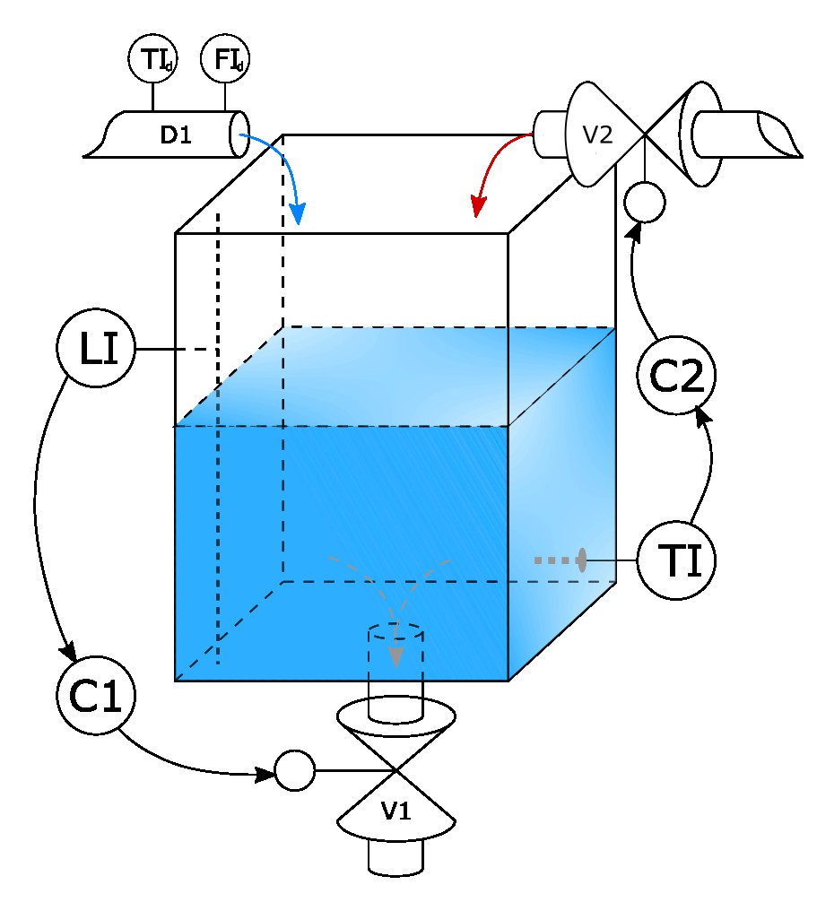
The process is a simple first principal model of a water tank. The tank dimensions in meters ($L \times W \times H$) are $0.5 \times 0.5 \times 1.5$. It has uncontrolled measured inlet water flow ($FI_d^1$) with measured temperature ($TI_d$). It is possible to manipulate tank water level $LI$ by setting position for the outlet valve $V_1$ between $0$ and $1$ ($0\ \%$ to $100\ \%$) and manipulate temperature inside tank $TI$ by setting position of hot water inlet valve $V_2$ in the same range. Valves opening/closing speed is limited to $0.02$ ($2\ \%/s$) as real world valves cannot be opened or closed immediately and have some traveling time. Both valves have linear characteristics meaning that valve position in per cents is equal to the area of the valve opening in per cent (e. g. if valve maximum opening area is $10\ cm^2$ then $30\ \%$ position means that opening area is $3\ cm^2$). At the same time water flow through the opening depends on the pressure before the valve. In case of valve $V_1$ the pressure depends on the water level in the tank – the higher is the level the bigger is the water flow through the same opening. This makes effect of $V_1$ to the process to be nonlinear. In case of $V_2$ it is assumed that pressure before valve is constant ($2\ bars$ or $200\ kPa$). Hot water temperature is fixed at the value of $90ºC$.

Identification data collection

Simulation step tests were manually generated to keep tank level in between minimum and maximum values.

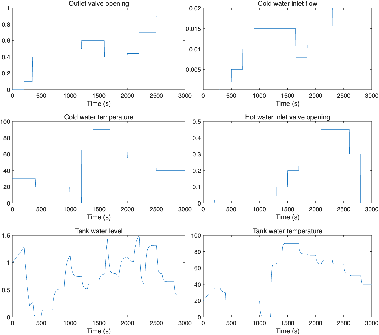
Inputs are: 1. Outlet valve posiotion; 2. Inlet flow; 3. Inlet temperature; 4. Inlet hot valve position.
Outputs are: 1. Tank level; 2. Tank temperature.

Input data generation script is generate_input_data.m. Data includes 3000 samples with $1s$ sample time.

Identification algorithm

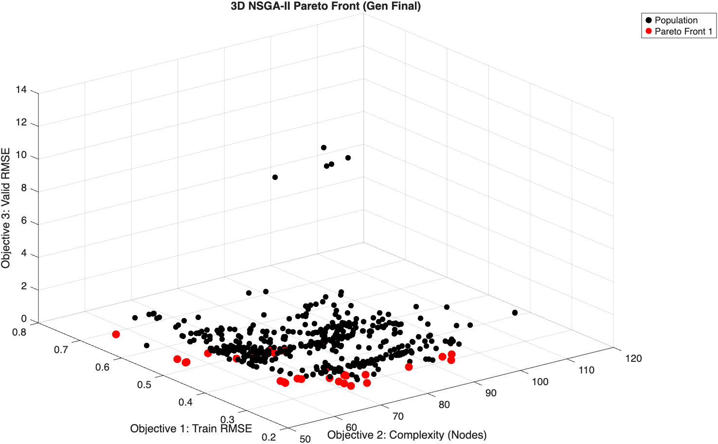
This code uses a Multi-Objective Genetic Programming (MOGP) algorithm (NSGA-II) distributed across an Island Model architecture to automatically discover the mathematical equations of a nonlinear state-space system from input-output data. It acts as a Grey-Box identifier by injecting known physical equations as protected structural seeds, and uses Memetic optimization (BFGS or Nelder-Mead) to continuously fine-tune the constants, ultimately finding the Pareto-optimal models that balance predictive accuracy (RMSE) against equation complexity (BIC).

Identitification exmample

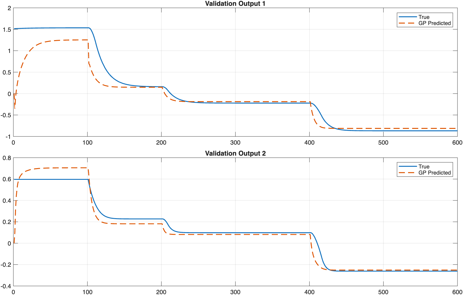
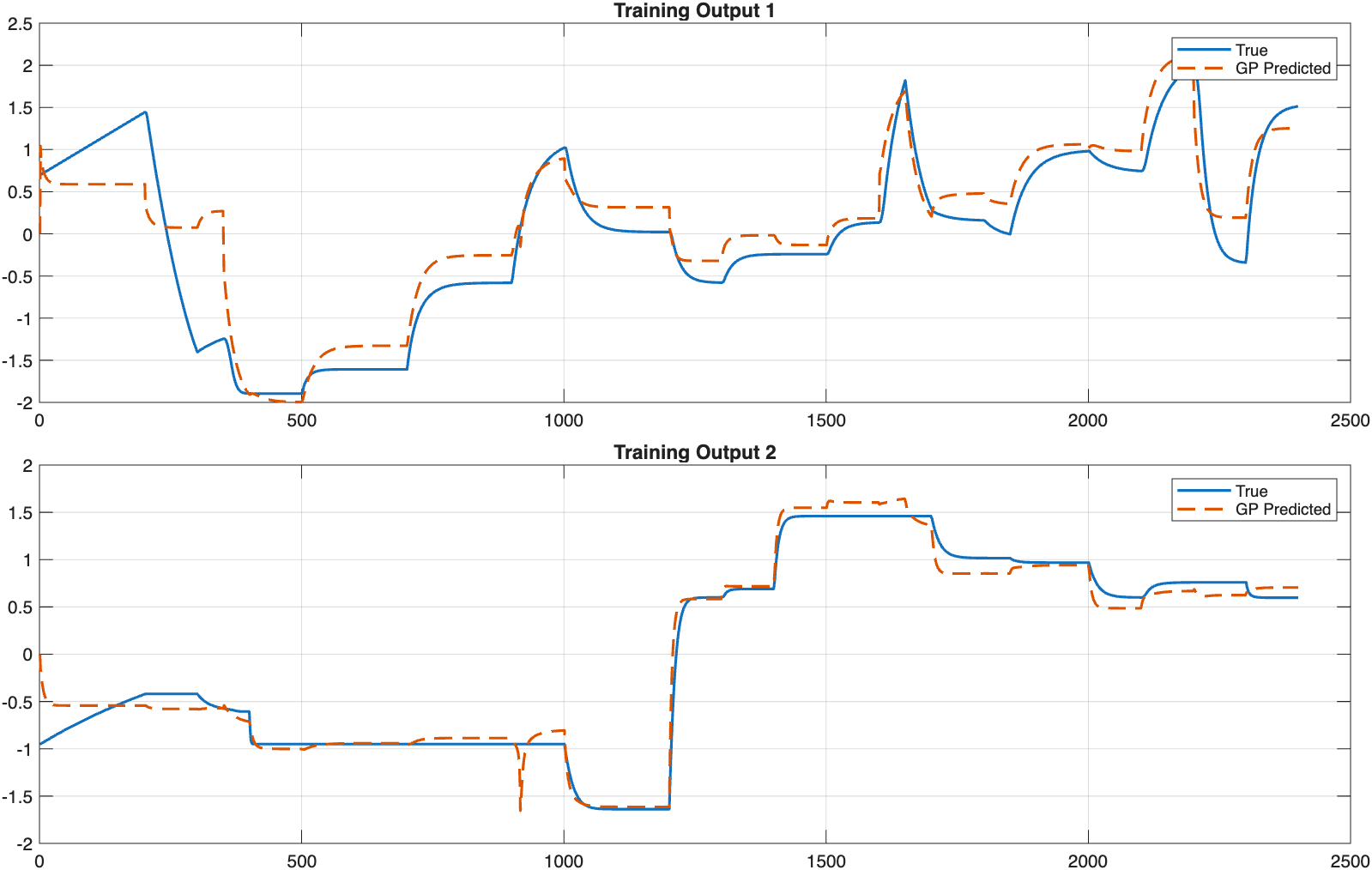
FINAL BEST MODEL: TrainRMSE=0.3004, ValRMSE=0.2073
Best expression trees:
State 1: $((0.95695 * x1) + (((-0.85714 * u2) + (-0.58294 * u4)) - ((-0.2216 * sqrt(x1)) * u1)))$
State 2: $((0.66682 * x2) + ((((0.78257 * u3) * u2) + (0.87099 * u4)) / (0.83938 * sqrt(x1))))$
State 3: $((-0.083961 * x3) + log(exp((u1 + -0.33523))))$
State 4: $((0.83303 * x4) + tanh((-0.050176 * u3)))$
Output Matrix C:

$$\begin{bmatrix} -0.0685 & 0.0555 & -0.4404 & 0.6286 \\ -0.0084 & 0.0971 & 0.0248 & -2.6538 \end{bmatrix}$$

1. Pareto Front

2. Training Data Fit

3. Validation Data Fit

Current architecture flowchart